Start learning JVM internals with Grafana dashboard

Table of Contents

Photo generated with Leonardo Ai

Are you a Java developer who knows the ins and outs of programming in Java but finds the world of JVM internals a bit mystifying? You’re not alone. Understanding what goes on under the hood of the Java Virtual Machine (JVM) can seem like a daunting task. In this blog post, I’ll demystify basic JVM internals concepts using insights from a popular Grafana dashboard. Buckle up, we’re going on an adventure into the JVM world!

Not enough memory #

Learning a programming language can be a challenging journey. First, you need to grasp the basic syntax to accomplish standard tasks. The next step involves learning one or two popular frameworks within a given ecosystem to enhance your visibility in the job market. However, once you secure that dream job, you quickly realize that having a solid foundation in a programming language and popular frameworks is not sufficient. Elements like best practices, design patterns, and system design play crucial roles in becoming a successful expert in software development.

Finally, a day arrives when you have mastered all this knowledge (or at least you think you have), and you receive a call from the operations team stating that your application is experiencing overwhelming success but struggles to handle the large influx of user requests. None of the previous steps prepared you for the skyrocketing CPU usage or memory issues. Panic sets in as you desperately try to recall why these components are essential and how they relate to your state-of-the-art application.

Look into inside #

Does it sound familiar?

How could you prevent this from happening? The first step is to come to the realization that you don’t know everything about your piece of software. Yes, you have coded it, but do you know how it behaves in the wild production environment? If you received a similar call, you probably don’t know. Therefore, the next step for you would be to initiate app monitoring to observe trends and receive alerts when key metrics approach dangerous thresholds. Additionally, understanding how the app responds under various types of pressure is crucial.

Numerous tools can be employed for this purpose. Some are built into the JDK, such as Java Flight Recorder with Java Mission Control, while others can be downloaded, like JProfiler, and some are cloud platforms, such as Datadog. It’s easy to feel overwhelmed initially, as each tool provides different types of information, often at a very low level.

So, where do you begin with monitoring app performance? Which tool should you choose first?

Grafana dashboard #

I would recommend starting with Prometheus and Grafana. Both tools are open source and non-invasive, meaning there’s no need to add any special tool/agent that may affect overall performance. They only require adding metrics libraries to a project. The setup is relatively straightforward, as I’ve outlined in a previous article - How to set up monitoring tools for JVM.

The mentioned post also covers how to import one of the most popular JVM dashboards - JVM (Micrometer) - which will be the subject of this post. It will walk you through key metrics and explain when and why they’re important.

The dashboard consists of sections that will be described in the following parts, which I’ve grouped and changed the order a little bit.

JVM Memory #

If you ever wonder what’s the first thing that you must keep eye on when monitoring Java application in most of the case it would be the memory usage. This is a vital information about the health of an app, since JVM needs it to run it.

Therefore it is not a suprise thet this is a first information that is provided by the dashboard - the percentage of how much heap and non-heap memory is fillied up (along with data about how long the app is running).

In most applications, these two metrics are the ones we should keep an eye on. They have a significant impact on its performance and can quickly explain why the app is running slow or even crashing.

Why these two metrics are that important? First of all we need to know that Java is object-oriented language. It means that every program is a set of objects which interact with each other. They have methods that are invoked by other objects and they also hold data. And in the real applications number of objects may be very large. And that’s why it is worth to monitor their number and size with the first indicator. The latter is accountable for measuring memory use of non-object related things, which in some cases are also worth to monitor.

Moving on, let’s examine the charts above, which illustrate how memory usage has changed over time. The charts depict the actual memory usage (used) at a given moment, the maximum available (max), and the memory guaranteed to be available for the JVM (committed).

What can we read from the Heap memory chart? Certainly, the used memory shouldn’t reach the max value. A dangerous situation arises when the increasing amount of memory in the Heap area indicates that many objects are created and never destroyed (collected by the Garbage Collector, which will be mentioned later). If this happens, the app will start to act slower and eventually crash, throwing the java.lang.OutOfMemoryError.

In addition to Heap data, the JVM has a second data area called Non-Heap (or Off-Heap or Native Memory). It stores various data, which can be divided into the following spaces:

Metaspace (aka Method Area): It holds class-related information about class code, their fields, and methods after being loaded by the classloader (more about it in the article). It also contains information about constants (in the Constant Pool).
Code Cache: This area stores optimized native code produced by the Just-In-Time compiler.
Program Counters: These point to the address of the currently executed instruction (each thread has its own Program Counter).
Stacks: The Last-In-First-Out (LIFO) stack of frames for each executed method. It contains primitive variables and references to the objects on the heap.

While it is typically the heap that may be too small, we need to understand that memory problems with non-heap data could also crash an app. Too many classes loaded into Metaspace may cause a java.lang.OutOfMemoryError, and too many frames in the Stack may result in a java.lang.StackOverflowError being thrown.

JVM Memory Pools (Heap) #

Let’s now delve into Heap usage. But first, we need to understand how the Heap is structured because it is not a monolith. The Heap is divided into various spaces, the number of which depends on the type of Garbage Collector used. Above, we can see three charts for Eden Space, Survivor Space, and Old Gen, which are used by the G1 Garbage Collector.

But why is the Heap split into spaces? It comes from something called the weak generational hypothesis. This hypothesis presumes that the lifespan of objects varies. Most of them are very short-lived, used only once, and then the memory they occupy can be freed. Others, usually a smaller fraction, are the ones that are constantly used and cannot be destroyed. Due to this fact, the Garbage Collector (GC) splits the heap into generations (spaces), where short-lived objects reside in young generations (Eden Space and Survivor Space), and long-lived objects in an old generation (Old Gen).

Having the heap split into generations allows the GC to avoid performing one long garbage collection on the entire heap. Instead, the GC performs it only on a subset at a time. It also allows for different collection frequencies in each generation; the Eden Space is cleaned more often than the Old Gen because objects located there are needed only for a short period.

The above screenshot confirms this. We can see that the plot for used memory in Eden Space is formed in a characteristic jigsaw pattern. It quickly fills up with new objects (expressed as a rising plot on the chart), and once it reaches a certain threshold, it is emptied (causing the plot to go down).

On the contrary, the Survivor Space and Old Gen are much more stable. There are some changes in them, but they are very subtle.

These three charts give us vital information about the content of the heap. We can read how often new objects are created and removed. If the cleanup for them is done very often and the old objects are kept at a relatively same level, it is tempting to increase the ratio of young to old generation size. The larger the young generation is, the less often cleanup will be done. But on the other hand, it will be bigger, so the cleanup may take a little bit longer. The same goes for old generations; the smaller it gets, the more frequently it is cleaned. So we must keep a balance of it.

To adjust it, use -XX:NewRatio=N (which is a ratio of young and old generations, e.g., N=2 means that the young generation is twice as big as the old one) or -XX:NewSize=N (which is the initial size of the young generation - all remaining will be assigned to the old generation).

What if the app is consuming too much memory? #

The heap is one of the most crucial memory areas for JVM and typically requires a substantial amount of space. If it approaches the maximum threshold, the simplest solution is to increase heaps’ maximum size. A larger heap ensures that all necessary objects can fit into it. This can be accomplished by specifying -Xmx followed by the size in megabytes allocated for the heap. For example, -Xmx1024m will allocate 1024 MB for the heap. It’s easy and straightforward.

While adjusting the maximum size of the heap may provide a temporary solution, in many cases, it merely masks the symptoms rather than addressing the root cause of the problem. An increasing number of objects could indicate a memory leak within the application, requiring identification and resolution in the code.

Another possibility is that an excessive amount of data is being loaded into memory, either due to an inefficient data structure or an unexpectedly large volume of it. In the former case, optimizing how data is stored in the JVM is the solution, while in the latter, considerations such as increasing the heap size or chunking the large amount of data into smaller pieces.

But how to spot if we have inefficient data structure? There are couple of signs and one of them is using objects with lots of fields (e.g. entities) from which only a small subset is used. Limiting the number of fields per task can be beneficial here. Also we need to remember that even if fields won’t be initialized they also consume memory!

Additionally, strive to avoid using objects instead of primitives. Many instances exist where objects contain fields like Boolean instead of plain boolean. While this may seem like a minor change, it can significantly impacts memory usage. Similarly, treating String objects as containers for numbers or booleans variables consumes more memory than necessary.

Another optimization to reduce memory footprint involves refraining from initializing String variables with identical values repeatedly.

In certain situations, it can be highly beneficial to avoid creating immutable objects. This is particularly true when new objects need to be created as copies of others. Of course, I’m not discouraging the use of immutable objects altogether, as they prove invaluable in many scenarios. However, for objects created and used within a small method once or twice, it is sometimes more advantageous to make them mutable.

These suggestions only scratch the surface of addressing memory-related issues. Numerous resources are available to guide you in further optimizing memory usage.

Garbage Collection #

The previous section already mentioned the Garbage Collector, which we will now examine more closely. It is a key component of the JVM because, in contrast to languages like C++, we, as developers, don’t need to worry about freeing memory once an object is no longer needed. The role of the GC is to decide which objects should be destroyed and which should be preserved.

All new objects are initially allocated in the Eden Space. However, during the next garbage collection, they are promoted to one of the Survivor Spaces if they are still in use. Subsequently, during subsequent garbage collections, they are again checked to determine whether they should be promoted to the next subspace of the Survivor Space or even to the Old Gen.

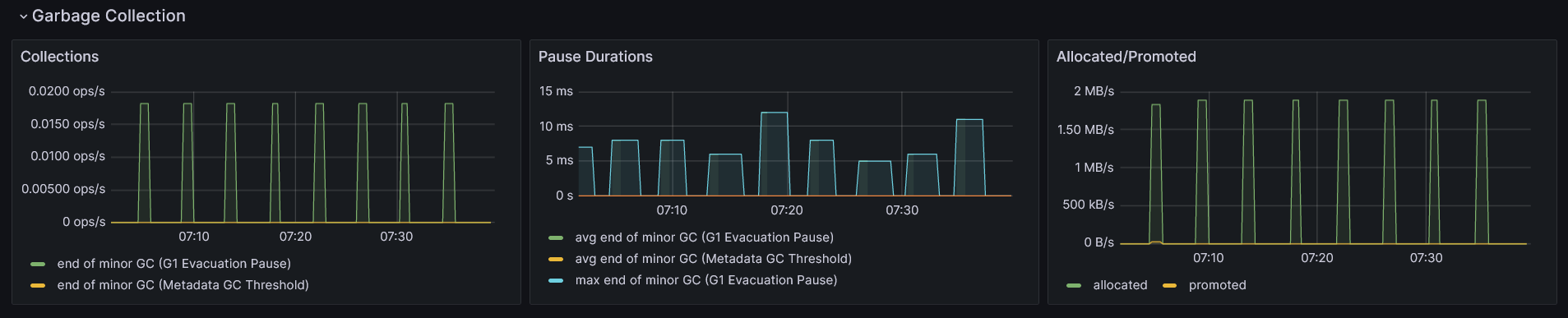
The first plot in the above screenshot, Collections, tells us how often a certain type of garbage collection occurs in a second. We can see that only one minor garbage collection (cleaning only the young generation of the heap) is happening, but it also shows a major garbage collection (cleaning objects from the old generation). By reading this chart, we can figure out how often each type of collection is occurring, and if it’s too frequent, it may suggest that one of the spaces is filling up too quickly with a large number of objects.

However, even if the number of collection occurrences is relatively high, it’s not always a cause for concern. If each one of them takes a very short time and does not significantly affect the overall application performance, we have nothing to worry about. To ensure that this is the case, we can look into the second plot, Pause Durations, which provides information about the average time of each garbage collection.

The last plot, Allocated/Promoted, shows us how much memory was used to allocate objects in the young generation and how much of it was promoted to older generations. This information is really helpful when we want to understand the memory load that GC needs to deal with in each cycle.

After identifying an issue in one of these graphs, we can take two approaches: tune JVM memory limits and GC behavior or select a different GC. Depending on the Java version and distribution (e.g., Oracle’s HotSpot, Amazon Corretto, Azul Zulu, or Eclipse Adoptium), the list of available GCs is different, but most of them can be categorized into:

Generational vs. non-generational - Some GCs may not split a heap into generations but treat it as a single memory space. However, usually it is not the case (though the approach varies among distributions).
Stop-the-world vs. concurrent - GCs in the first group pauses the entire application for cleanup, while the latter performs cleanup while the application is still running (or, to be precise, they briefly stop the application).
Single-thread vs. multi-thread - The first group operates using only one thread, while the latter utilizes at least two.
Incremental vs. monolithic - This is specific to stop-the-world GCs and indicates whether garbage collection is done only for a subset of the generation or until it’s complete.

Here is a list of available GCs in the Amazon Corretto distribution of OpenJDK, one of the most popular distributions according to the 2023 State of the Java Ecosystem for 21 version of Java:

Garbage Collector	Generational	Concurrent	Multi-thread	Monolithic	Purpose
G1	✅ Yes	✅ Yes (partially)	✅ Yes	✅ Yes	Common purpose GC, default
Serial	✅ Yes	❌No	❌No	✅ Yes	Good for apps with small heap
Parallel	✅ Yes	❌No	✅ Yes	✅ Yes	Good for batch processing apps, where overall throughput can be traded for longer pauses
Shenandoah	❌No	✅ Yes	✅ Yes	❌No	Reduces GC pauses
Generational ZGC	✅ Yes	✅ Yes	✅ Yes	❌No	For apps that needs short response time and large heap

The above table lists all available GCs along with their basic properties. Even though some of them may seem better than others, it is crucial not to overlook trade-offs. For instance, the short garbage collection pauses of Shenandoah and ZGC come with the cost of higher CPU usage. Therefore, before selecting one, make sure you understand the price you would need to pay.

If you are looking for more information about each GC, check the References section, where I’ve included links to the official documentation of each one of them.

JVM Memory Pools (Non-Heap) #

Apart from objects, JVM needs memory to store other things. This is represented by the next graphs from JVM Memory Pools (Non-Heap) in the discussed dashboard.

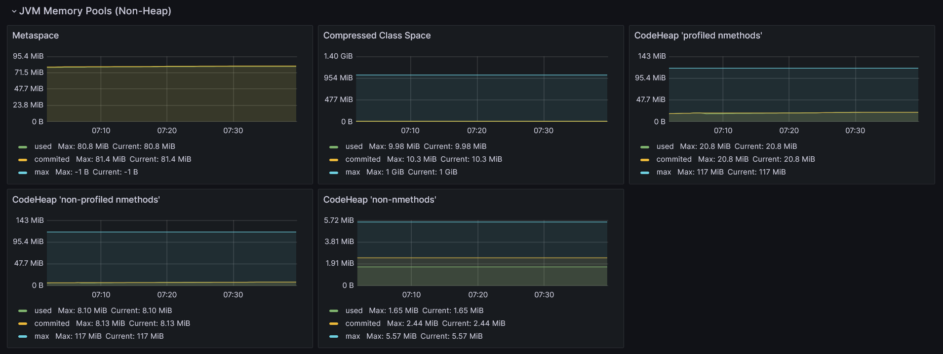
Metaspace (a.k.a. Method Area) - This is the place where metadata and definitions of every class are stored (in simpler terms, every .class file in the runtime representation). Additionally, Metaspace holds method counters used by the JIT compiler and a constant pool (a data structure to store information about references and constants associated with a class, such as static final fields). By default, there are no limits on how big it can get, but it can be tuned using the -XX:MaxMetaspaceSize flag. If not provided, it may occur that the JVM will consume too much memory and slow down the machine on which the application is running.
Compressed Class Space - This is a subset of Metaspace with classes metadata.

The remaining three graphs show segments of the code cache. It is used to store code optimized by the JIT (Just-In-Time) compiler. This compiler plays a vital role in JVM by identifying and optimizing places in the code that are executed very often. These hot spots (hence the name HotSpot for Oracle’s JDK distribution) are identified and recompiled from bytecode to machine (native) code. Along with other optimizations, such as method inlining or dead code elimination, it makes those parts of the code ultra-fast to execute, making Java applications robust.

Code cache is split into three segments:

CodeHeap ‘profiled nmethods’ - This segment holds lightly optimized methods.
CodeHeap ’non-profiled nmethods’ - This segment contains fully optimized methods.
CodeHeap ’non-nmethods’ - The smallest segment that contains compiler buffers and the bytecode interpreter.

This provides all the insights that the discussed dashboard gives us about the non-heap area. While these are valuable pieces of information, it’s crucial to be aware that it’s not everything. All mentioned data areas, like the heap and parts of the non-heap, are shared among all application threads. However, some areas are assigned to specific threads, such as the stack or program counter, and these are also vital parts of the JVM.

Classloading #

Besides information about the amount of memory occupied by loaded classes, the dashboard also provides details on how many classes were loaded into memory and when these loadings occurred. This information can be gleaned from the first two charts:

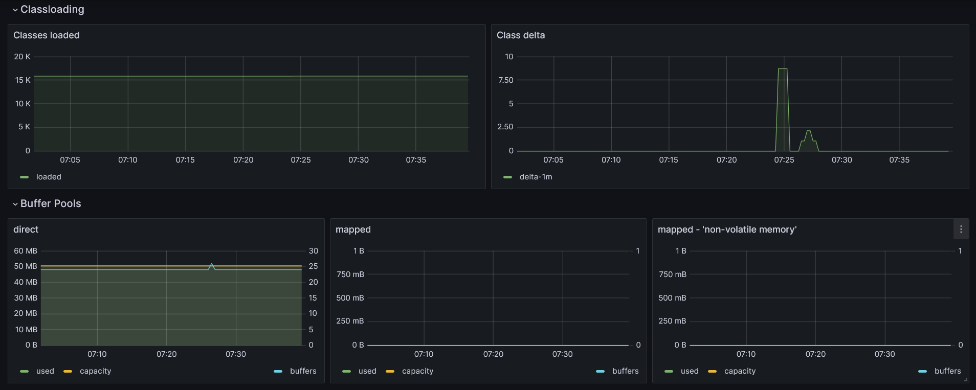
Most of the class loading occurs during the application startup, especially for solutions utilizing Inversion of Control. This is when most objects need to be initialized, preceded by the loading of their definitions into the JVM process. However, not all classes are loaded immediately. Some class definitions are loaded lazily during runtime

JVM Misc #

Next section available in the dashboard govers various things worth monitoring.

The name of the first chart, CPU Usage, suggests that it shows how the CPU is utilized. It presents three series: system (total CPU usage of the host), process (CPU usage for all JVM processes), and process-15m, which is an average of the latter gauge from the last 15 minutes.

The next graph, Load, provides more insight into the number of processes (load) running and queued for the CPU on average in 1 minute. If this indicator is below the number of available CPUs (also available on this chart), it means that there are no waiting processes due to occupied CPU, which is good news. Otherwise, it would indicate that the CPU can’t keep up with executing all processes.

The next two graphs provide information about JVM threads. The first one, Threads, displays the number of daemon threads, which are the opposite of user threads. Essentially, these two types of threads in the JVM are almost the same. The first difference is that when the program is stopped, first the user threads are halted, and then the daemon threads are exited. Only after that is the JVM considered as non-running. The second difference is that daemon threads serve the user thread. Typically, they are assigned to handle garbage collection, but they can also be utilized in our code by marking the Thread object with the setDaemon(true) methods.

The second graph, Thread States, presents the distribution of threads divided by their state.

The next row of charts starts with GC Pressure, indicating the percentage of CPU used for garbage collection. It’s essential to monitor this metric along with other garbage collection metrics mentioned earlier.

Another noteworthy metric to keep an eye on is the number of logs produced by the app, grouped by level, known as Log Events. This information can be valuable for spotting problems if the number of warn or error level logs is higher than usual, which may not be apparent in other metrics.

The last chart, File Descriptors, displays the number of files opened by the process.

I/O Overview #

The last section provides data not directly connected with JVM, but it’s crucial to keep an eye on, especially if it provides a REST API (which is the case for most Java applications nowadays).

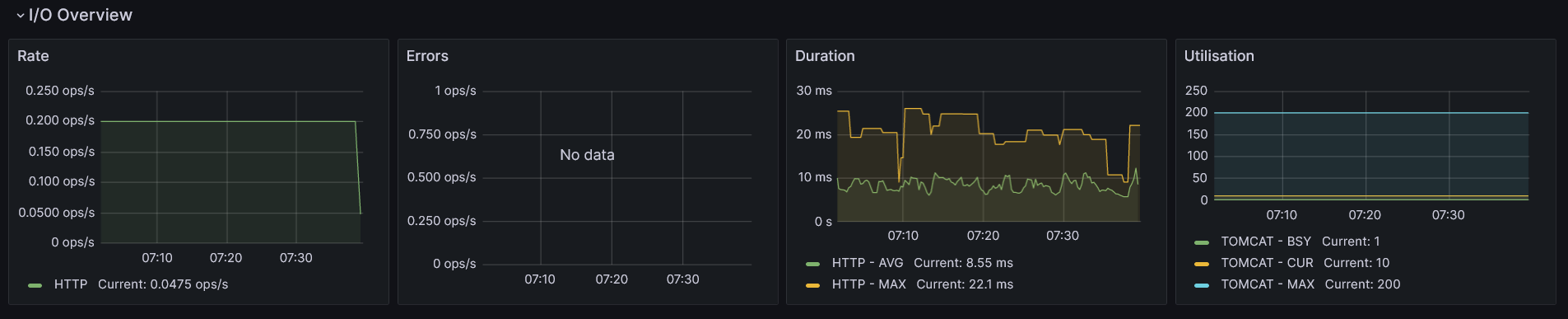
The first chart shows how many HTTP requests per second were made. The next one provides the same information, but this time narrowed down to all 5xx responses. A significant increase in 5xx responses may indicate unwanted issues. Also, in the case of high user traffic (as indicated in the first chart), it’s worth monitoring how much memory is consumed by the app, how often garbage collection is performed, or other indicators mentioned earlier. All of these factors may be correlated and affect how fast users receive a response from your service.

The next indicator measures how much time, on average and at maximum, HTTP requests took (excluding 5xx responses). A sudden increase in this metric may indicate that garbage collection pauses are taking longer than usual, which is worth checking in that case.

The last chart provides information about Tomcat’s (or Jetty’s) busy and active threads. It shows how many of them are currently in use, which is crucial for understanding the throughput of an application. The chart also displays information about the configured maximum number of Tomcat’s threads. If the number of currently used threads is very close to this limit, it should serve as a warning that the application may not be able to handle all incoming requests.

Conclusion #

And there you have it! 🚀 We’ve journeyed through the entire JVM (Micrometer) Grafana dashboard and soaked in a ton of insights about the JVM and its crucial indicators. 🧠✨ I hope that now the JVM feels more like a friendly companion than a mysterious black box. If you’re hungry for more knowledge, check out the references mentioned below or dive into tools like Java Flight Recorder or profilers. 🛠️ Who knows, maybe they’ll make an appearance on this blog someday!

Until then, why not set up the Grafana dashboard for your project and start unveiling the secrets of how your software dances in the production environment? Happy monitoring! 🎉👩‍💻👨‍💻